![[Experimental]](figures/lifecycle-experimental.svg)
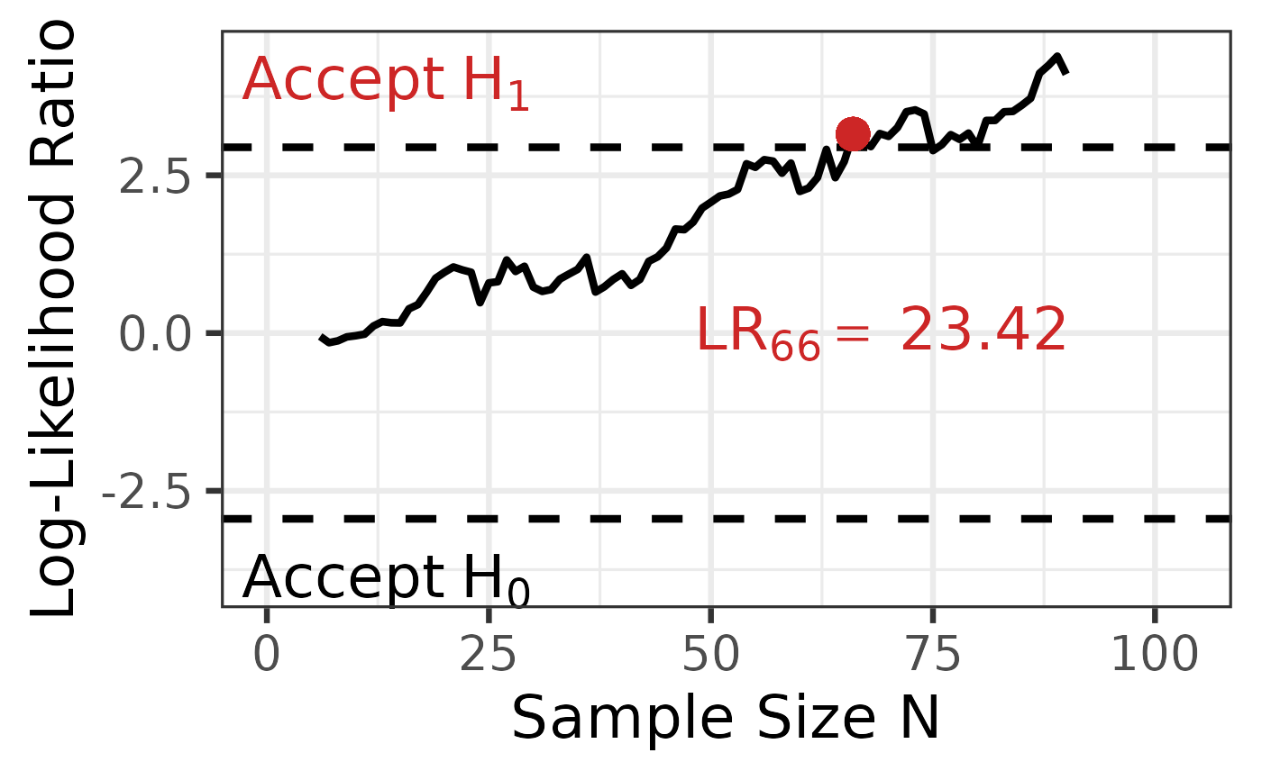
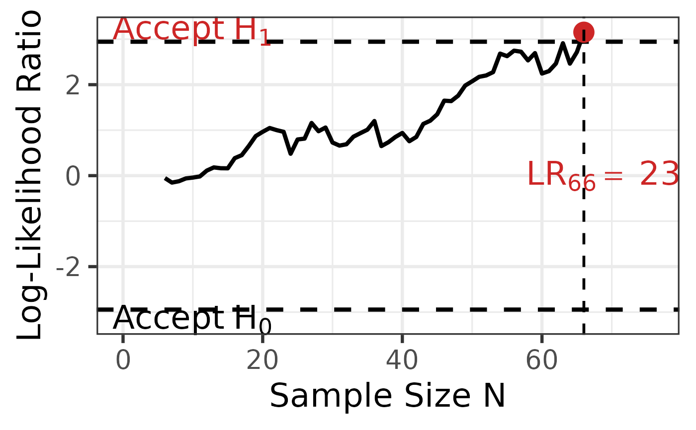
Creates a visualization of the sequential probability ratio test (SPRT) for ANOVA results, showing the log-likelihood ratio trajectory across sample sizes and decision boundaries.
Usage
plot_anova(
  anova_results,
  labels = TRUE,
  position_labels_x = 0.15,
  position_labels_y = 0.1,
  position_lr_x = NULL,
  position_lr_y = NULL,
  font_size = 15,
  line_size = 1,
  highlight_color = "#CD2626"
)
Arguments
- anova_results
A
seq_anova_resultsobject fromseq_anova(). Important: Theseq_anova()function must be called withplot = TRUEto generate the necessary data for plotting.- labels
Logical. If
TRUE(default), display decision labels ("Accept H0" / "Accept H1") and the likelihood ratio at the decision point.- position_labels_x
Numeric value between 0 and 1 controlling the horizontal position of decision labels as a proportion of maximum sample size. Default is
0.15(left side);0.5centers the labels.- position_labels_y
Numeric value controlling the vertical spacing between decision boundaries and their labels. The value is multiplied by
max(|log-likelihood ratio|)to determine spacing. Larger values move labels further from boundaries. Default is0.075.- position_lr_x
Optional numeric value for the x-coordinate (sample size) of the likelihood ratio label. If
NULL(default), positioned at the decision point or final sample size.- position_lr_y
Optional numeric value for the y-coordinate (log-likelihood ratio) of the likelihood ratio label. If
NULL(default), positioned aty = 0for early decisions, or slightly offset for continuing sampling scenarios.- font_size
Numeric. Base font size for plot text. Default is
20.- line_size
Numeric. Line width for the trajectory and boundaries. Default is
1.5.- highlight_color
Character string. Color for highlighting the decision point or final sample. Default is
"#CD2626"(red).
Value
A ggplot2::ggplot() object showing:
Log-likelihood ratio trajectory across sample sizes
Dashed horizontal lines indicating decision boundaries
Highlighted point showing where decision was reached (or final sample)
Optional labels for decision regions and likelihood ratio value
Examples
# simulate data for the example ------------------------------------------------
set.seed(3)
data <- sprtt::draw_sample_normal(3, f = 0.25, max_n = 50)
# calculate the SPRT -----------------------------------------------------------
anova_results <- sprtt::seq_anova(y~x, f = 0.25, data = data, plot = TRUE)
# plot the results -------------------------------------------------------------
# default settings
sprtt::plot_anova(anova_results)
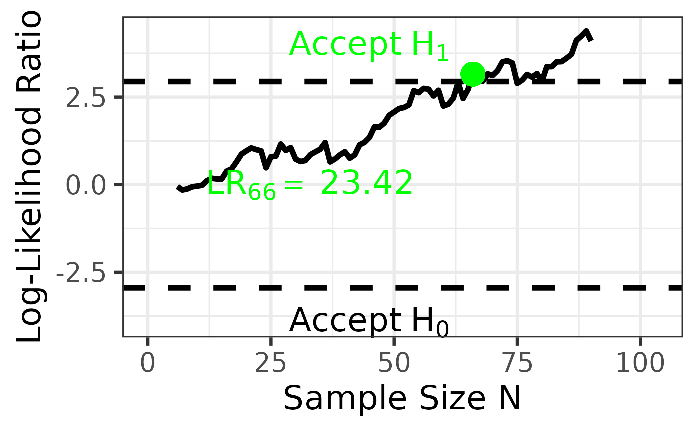
 # variant 1
sprtt::plot_anova(anova_results,
labels = TRUE,
position_labels_x = 0.05,
position_lr_x = 150,
position_lr_y = 0,
highlight_color = "green"
)
# variant 1
sprtt::plot_anova(anova_results,
labels = TRUE,
position_labels_x = 0.05,
position_lr_x = 150,
position_lr_y = 0,
highlight_color = "green"
)
 # variant 2
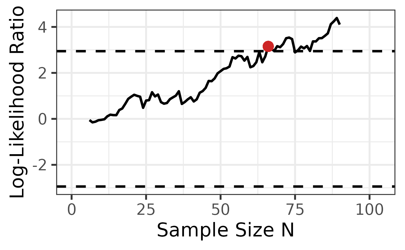
sprtt::plot_anova(anova_results,
labels = TRUE,
position_labels_x = 0.15,
position_labels_y = 0.2,
position_lr_x = 60,
position_lr_y = 1,
font_size = 25,
line_size = 2,
highlight_color = "darkred"
)
# variant 2
sprtt::plot_anova(anova_results,
labels = TRUE,
position_labels_x = 0.15,
position_labels_y = 0.2,
position_lr_x = 60,
position_lr_y = 1,
font_size = 25,
line_size = 2,
highlight_color = "darkred"
)
 # no labels
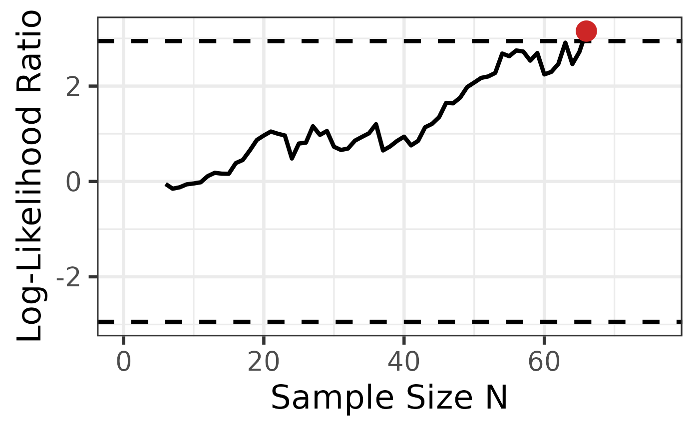
sprtt::plot_anova(anova_results,
labels = FALSE
)
# no labels
sprtt::plot_anova(anova_results,
labels = FALSE
)
 # custom additions
sprtt::plot_anova(anova_results) +
ggplot2::geom_vline(xintercept = 66, linewidth = 1, linetype = "dashed")
# custom additions
sprtt::plot_anova(anova_results) +
ggplot2::geom_vline(xintercept = 66, linewidth = 1, linetype = "dashed")
 # further information ----------------------------------------------------------
# run this code:
vignette("one_way_anova", package = "sprtt")
#> Warning: vignette ‘one_way_anova’ not found
# further information ----------------------------------------------------------
# run this code:
vignette("one_way_anova", package = "sprtt")
#> Warning: vignette ‘one_way_anova’ not found